Plotting mechanics and EDA

Run the code below, and read along.

In the last assignment, I gave you a list of firms from 2020 with variables

• “gvkey”, “lpermno”, “lpermno” = different datasets use different identifiers for firms
• “fyear” = the fiscal year the remaining variable apply to
• “gsector” = gsector, an industry classification (see the wiki article on GICS)
• “state” = of headquarters
• “tic” = ticker
• various accounting statistics

This data is a small slice of Compustat, which is a professional grade dataset that contains accounting data from SEC filings.

We downloaded it and found a subsample of firms that we were interested in:

import pandas as pd
import numpy as np
import seaborn as sns
import pandas_datareader as pdr  # to install: !pip install pandas_datareader
from datetime import datetime
import matplotlib.pyplot as plt 
import yfinance as yf

plt.rcParams['patch.edgecolor'] = 'none' 

# this file can be found here: https://github.com/LeDataSciFi/ledatascifi-2021/tree/main/data
# if you click on the file, then click "raw", you'll be at the url below,
# which contains the raw data. pandas can download/load it without saving it locally!
url = 'https://github.com/LeDataSciFi/data/raw/main/Firm%20Year%20Datasets%20(Compustat)/firms2020.csv'
firms_df = pd.read_csv(url).drop_duplicates('tic') 

# add leverage 
firms_df['leverage'] = (firms_df['dlc']+firms_df['dltt'])/firms_df['at']

# high_lev = 1 if firm is above the median lev in its industry
firms_df['ind_med_lev'] = firms_df.groupby('gsector')['leverage'].transform('median')
firms_df.eval('high_leverage = leverage > ind_med_lev',inplace=True)

# problem: if lev is missing, the boolean above is false, so 
# high_lev = false... even if we don't know leverage!
# let's set those to missing (nan)
mask = (firms_df["leverage"].isnull()) | (firms_df["ind_med_lev"].isnull())
firms_df.loc[mask,"high_leverage"] = None

# reduce to subsample: (has leverage value and in our sectors)
subsample = firms_df.query('gsector in [45,20] & (high_leverage == 1 | high_leverage == 0)') 
ticker_list = subsample['tic'].to_list()

Now,

1. I will download their daily stock returns,
2. Compute (EW) portfolio returns,
3. Using (2), compute weekly total returns (cumulate the daily returns within each week).
   • Note: These are not buy-and-hold-returns, but rather daily rebalancing!
   • If you want buy-and-hold returns, you’d compute the weekly firm level returns, then average those compute the portfolio returns.

##################################################################
# get daily firm stock returns
##################################################################

# I called this first df "stock_prices" in the last assignment

firm_rets   = (yf.download(ticker_list, 
                           start=datetime(2020, 2, 2), 
                           end=datetime(2020, 4, 30),
                           show_errors=False)
                .filter(like='Adj Close') # reduce to just columns with this in the name
                .droplevel(0,axis=1) # removes the level of the col vars that said "Adj Close", leaves symbols
               
                # reshape the data tall (3 vars: firm, date, price, return)
                .stack().swaplevel().sort_index().reset_index(name='Adj Close')
                .rename(columns={'level_0':'Firm'})
 
                # create ret vars and merge in firm-level info
                .assign(ret = lambda x: x.groupby('Firm')['Adj Close'].pct_change())
                .merge(subsample[['tic','gsector','high_leverage']],
                       left_on='Firm',
                       right_on='tic')
               
               )
 
##################################################################
# get daily portfolio returns
##################################################################

# these portfolio returns are EQUALLY weighted each day (the .mean())
# this is as if you bought all the firms in equal dollars at the beginning 
# of the day, which means "daily rebalancing" --> each day you rebalance
# your portfolio so that it's equally weighted at the start of the day

daily_port_ret = (firm_rets
                  # for each portfolio and for each day
                  .groupby(['high_leverage','gsector','Date']) 
                  ['ret'].mean()                       # avg the return for that day for the firms in the port
                  .reset_index()                       # you can work with high_leverage/sector/date as index or vars
                                                       # I decided to convert them to variables and sort                                                    
                  .sort_values(['high_leverage','gsector','Date'])
                 )

##################################################################
# get weekly portfolio returns
##################################################################

# we will cumulate the daily portfolio returns so now we have a  
# dataframe that contains weekly returns for a few different portfolios

weekly_port_ret = (daily_port_ret
                   # compute gross returns for each asset (and get the week var)
                   .assign(R = 1+daily_port_ret['ret'],
                           week = daily_port_ret['Date'].dt.isocalendar().week.astype("int64"))
                   
                   # sidenote: dt.isocalander creates a variable with type "UInt32"
                   # this doesn't play great with sns, so I turned it into an integer ("int64")
                   
                   # for each portfolio and week...
                   .groupby(['high_leverage','gsector','week'])
                   # cumulate the returns
                   ['R'].prod()
                   # subtract one
                   -1
                  ).to_frame()
                   # this last line above (to_frame) isn't strictly necessary, but 
                   # the plotting functions play nicer with frames than series objs

[*********************100%***********************]  388 of 388 completed

Our first plot

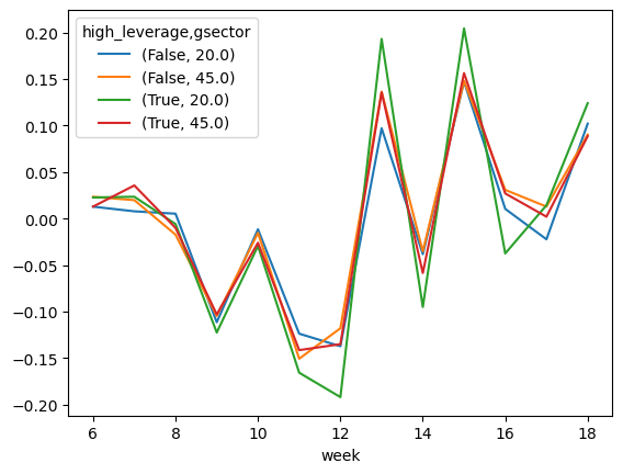
We can plot the weekly potfolio returns easily.

ax = weekly_port_ret.squeeze().unstack().T.plot()
# can access customization via matplotliab methods on ax 
plt.show()

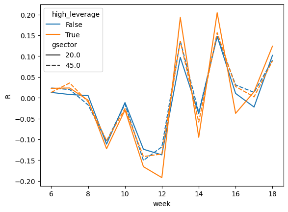
Doing this in seaborn is easy too.

ax = sns.lineplot(data = weekly_port_ret,
             x='week',y='R',hue='high_leverage',style='gsector')
# can access customization via matplotlib methods on ax 
plt.show()

Part 1 - Plot formatting

Insert cell(s) below this one as needed to finish this Part.

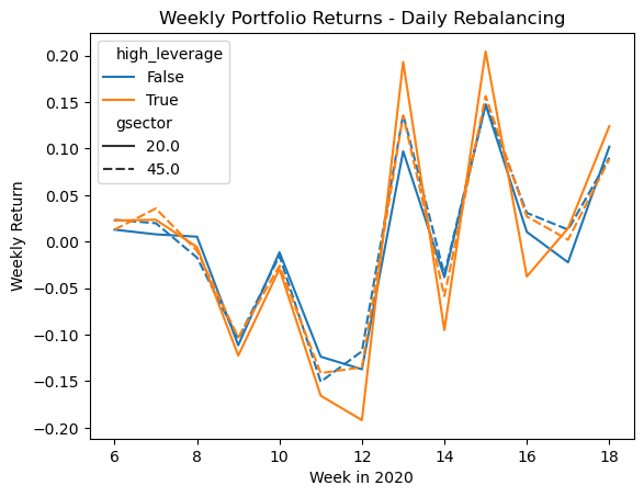
Improve the plot above.

• Q1: set the title to “Weekly Portfolio Returns - Daily Rebalancing”
• Q2: set the x-axis title to “Week in 2020”
• Q3: set the y-axis title to “Weekly Return”
• Q4: Ungraded bonus challenge: change the legend so it says the industry names, not the numbers

ax = sns.lineplot(data = weekly_port_ret,
             x='week',y='R',hue='high_leverage',style='gsector')
# Q1
plt.title("Weekly Portfolio Returns - Daily Rebalancing")
# Q2
plt.xlabel("Week in 2020")
# Q3
plt.ylabel("Weekly Return")
# Q4

plt.show()

Part 2 - Replicate/Imitate

Insert cell(s) below each bullet point and create as close a match as you can. This includes titles, axis numbering, everything you see.

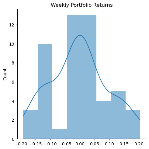
• Q5: Replicate F1.png. Notice the x-axis has no label - it’s in the title.

Q5_plot=sns.displot(data=weekly_port_ret,x='R',kde=True)
Q5_plot.set(xlabel=None)
plt.title('Weekly Portfolio Returns')
plt.show()

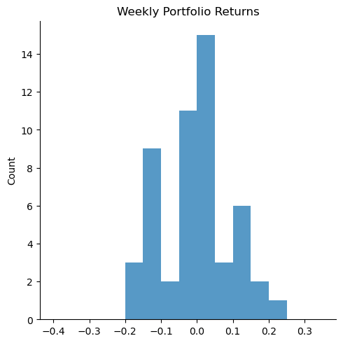
• Q6: Replicate F2.png. Notice the bin sizes are 5%.

Q6_plot=sns.displot(data=weekly_port_ret,x='R',bins=np.arange(-0.4, 0.4, 0.05))
Q6_plot.set(xlabel=None)
plt.title('Weekly Portfolio Returns')
plt.show()

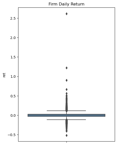
• Q7: Replicate F3.png. Pay attention to the header for a clue!

plt.figure(figsize=(5, 7)) 
sns.boxplot(y='ret', data=firm_rets, color='steelblue')
plt.title('Firm Daily Return')
plt.show()

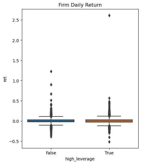
• Q8: Replicate F4.png. Pay attention to the header for a clue!

plt.figure(figsize=(5, 6)) 
sns.boxplot(x='high_leverage', y='ret', data=firm_rets)
plt.title('Firm Daily Return')
plt.show()

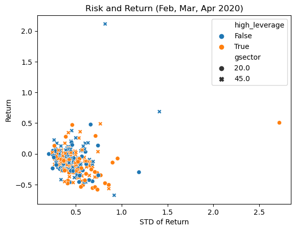
• Q9: Replicate this figure, using this total dataset:

total = pd.DataFrame() # open an empty dataframe
total['ret'] = (firm_rets.assign(ret=firm_rets['ret']+1) # now we have R(t) for each observation
                       .groupby('tic')['ret']    # for each firm,
                       .prod()                      # multiple all the gross returns
                       -1                           # and subtract one to get back to the total period return
)
total['cnt'] = firm_rets.groupby('tic')['ret'].count()
total['std'] = firm_rets.groupby('tic')['ret'].std()*np.sqrt(total['cnt'])
total = total.merge(firm_rets.groupby('tic')[['high_leverage','gsector']].first(), 
                    left_index=True, right_index=True)

total = pd.DataFrame() # open an empty dataframe
total['ret'] = (firm_rets.assign(ret=firm_rets['ret']+1) # now we have R(t) for each observation
                       .groupby('tic')['ret']    # for each firm,
                       .prod()                      # multiple all the gross returns
                       -1                           # and subtract one to get back to the total period return
)
total['cnt'] = firm_rets.groupby('tic')['ret'].count()
total['std'] = firm_rets.groupby('tic')['ret'].std()*np.sqrt(total['cnt'])
total = total.merge(firm_rets.groupby('tic')[['high_leverage','gsector']].first(), 
                    left_index=True, right_index=True)

total

	ret	cnt	std	high_leverage	gsector
tic
AAPL	-0.065597	60	0.348535	True	45.0
ABM	-0.064676	60	0.426696	False	20.0
ACLS	0.048741	60	0.557596	False	45.0
ACM	-0.225210	60	0.438323	False	20.0
ACN	-0.093329	60	0.347341	False	45.0
...	...	...	...	...	...
XRX	-0.468449	60	0.473751	True	45.0
XYL	-0.111853	60	0.371912	True	20.0
YELL	-0.254464	60	0.671546	True	20.0
ZBRA	0.009977	60	0.388039	True	45.0
ZS	0.172650	60	0.383923	True	45.0

342 rows × 5 columns

sns.scatterplot( x="std", y="ret", data=total, hue='high_leverage',style = 'gsector')
plt.legend(loc='upper right')
plt.title("Risk and Return (Feb, Mar, Apr 2020)")
plt.xlabel("STD of Return")
plt.ylabel("Return")
plt.show() 

Q10: Choose your adventure. Some ideas:

• Use a pairplot, jointplot, or heatmap on any data already loaded on this page (including the original firms_df).
• Convert any of the stock price datasets to a “wide” format and then use the pair_hex_bin code from the communiy codebook.
• Do something fun with the parameters of the function you choose.
• Or adapt this to improve our portfolio returns plot from Part 1, because Part 1 created a tough to interpret “spaghetti” plot!
• Plot the cumulative returns over the sample period for the four portfolios’ weekly returns from Part 1
• Adapt this to improve our weekly portfolio returns plot from Part 1.

Then save the figure as a png file and share it here on the discussion board.

sns.set_theme(style="dark")

# Plot each year's time series in its own facet
g = sns.relplot(
    data=weekly_port_ret,
    x="week", y="R", col="gsector", hue="high_leverage",
    kind="line", palette="crest", linewidth=1, zorder=6,
    col_wrap=2, height=3, aspect=1.5, legend=True,
)

# Iterate over each subplot to customize further
for year, ax in g.axes_dict.items():
    # Plot every year's time series in the background
    sns.lineplot(
        data=weekly_port_ret, x="week", y="R", units="high_leverage",
        estimator=None, color=".7", linewidth=1, ax=ax,
    )

# Tweak the supporting aspects of the plot
g.set_titles("Weekly Portfolio Returns")
g.set_axis_labels("Weeks", "Returns")
g.tight_layout()